The Networked SIR model

In the previous post we introduced the SIR model, and argued that a networked model might be more appropriate if one seeks to relax the assumption, that transmission of a pathogen can occur from any individual in the \(I\) compartment, to any individual in the \(S\) compartment (with the compartments viewed as sets of individuals instead of counts), and instead only is possible if there exists an edge, or symmetric relation between the individuals in a network that models the social interactions of a population of size \(N\).

This of course introduces the new assumption, that the network is a useful model of the social interactions (over the duration of the epidemic, in case of a static network, which we will assume the network is).

In this post I will show (with R code) how to perform stochastic simulations of a networked SIR model using the Gillespie algorithm [Gillespie, 1977], while representing the network using the igraph package.

Introduction

The networked SIR model is treated in e.g. [Kiss et al., 2017], and assumes that transmission of a pathogen, from an infected to a connected susceptible individual, takes place as a Poisson process with rate \(\hat \beta\) — the per-edge transmission rate, while recovery of an infected individual takes place as a Poisson process with rate \(\gamma\), independent of the network.

So, if a susceptible individual \(s_j \in S, \; j \in \{1,2,\ldots,N\} \) has \(n_j \in \mathbb N,\; 0 \leq n_j \leq N-1\) infected neighbours, then transmission to \(s_j\) takes place as a Poisson process with rate \( \lambda_j = n_j\,\hat \beta\).

A Poisson process is characterized by its exponentially distributed waiting times between events.
Let \( \tau_j \) denote the waiting time until \(s_j\) (with \(n_j\) infected neighbours) becomes infected, then \(\tau_j \) is exponentially distributed with density

\[ f_{\tau_j}(t;\,\lambda_j) = \lambda_j\,\exp^{-\lambda_j\,t} = n_j\,\hat \beta \,\exp^{-n_j\,\hat \beta\,t} \]

If at some time \(t \geq 0\) we have \(s_j,s_k \in S \), and \(s_j,s_k\) have infected neighbours. Then which individual gets infected first?
This is a case of so-called racing exponentials, and it turns out that the probability \( P(s_j\, \text{is infected first})=\frac{\lambda_j}{\lambda_j + \lambda_k} \), i.e. proportional to the rate, and similarly for \(s_k\). This fact is utilized in the Gillespie algorithm.

The Gillespie algorithm

The Gillespie algorithm was initially invented in order to perform stochastic simulations of chemical reaction systems, given by deterministic reaction-rate ODEs. Gillespie argued that stochastic effects could result in chemical reactions having realizations that were far from what the deterministic models predicted, and thus advocated using stochastic simulations as a complementary tool in conjunction with classical deterministic models when working with chemical reaction systems.

We will not concern ourselves with these academic discussions, but rather focus on using the Gillespie algorithm to simulate the networked SIR model.

We do this by simply considering infection and recovery events, instead of chemical reaction events, since both types of systems assume exponentially distributed waiting times between events. Then all that is required, is that we identify which types of events that can occur, and their rate.

Say we have \(m\) types of events. At the core of the Gillespie algorithm is the joint distribution

\[ P(\tau,j),\qquad \tau \in \mathbb R,\; j \in \{1,2,\ldots,m\} \]

which is the probability, given the state of the system at time \(t\), that the next event will occur at time \(t+\tau \), and will be an event of type \(j\).
It turns out that we can sample from this distribution first by sampling \(\tau\) from an exponential distribution with rate \(\lambda\) — the sum of all event rates at time \(t\), i.e. \( \lambda = \sum_{j=1}^m \lambda_j \), and then sample the type of event \(j\) with probability proportional the event rate \(\lambda_j,\; j \in \{1,2,\ldots,m\}\).
But we are getting ahead of ourselves! We first need a network of individuals...

Network representation

We can use the igraph package in R to represent the network of individuals in the networked SIR model.
Every individual in the population of size \(N\) is represented by a vertex in the network. The question is now: What is the topology of this network? Do we have to painstakingly construct this network by hand or what?
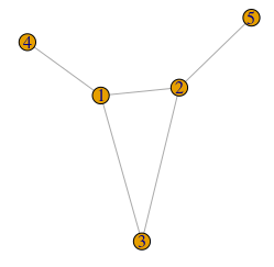
Random graphs to the rescue! Unless we want to use a real-world network, we simply sample the network uniformly from the set of connected networks with a specified degree sequence, which as the term suggests, gives the degree (number of connections) of all the vertices. We can do this with igraph package using the degree.sequence.game function. For example:

library(igraph)

seq <- c(3,3,2,1,1) # Degree sequence
G <- degree.sequence.game(seq, method="vl")
plot(G)

Plot of an example network with prescribed degree sequence seq produced by the code snippet above.

Note that the degree sequence needs to be graphical, i.e. the sequence sum needs to be even, and realizable as a simple graph — this can be determined using the Havel-Hakimi algorithm (Wikipedia).

So, if we have an assumption on the degree distribution of the population, from which the degree sequence can be sampled, then we can, given that the degree sequence is realizable, get a igraph object \(G\) that we can use in the implementation of the stochastic simulation.

Simulation code

In the implementation below we have a state vector \(X\) of length \(N\). The entries in the state vector can take on the values 0,1 or 2, corresponding to a susceptible, infected or recovered individual.
We also have a vector of rates \(\lambda\) of length \(N\), where some entries may be zero, depending on the state of the corresponding individual, and the state of the neighbours.
After initialization we sample the joint distribution \(P(\tau, j)\) mentioned above, and update \(X\) to reflect the new state of the system as a result of event \(j\). We also update the rates that are affected by this new state, i.e. some susceptible individuals may have more or fewer infected neighbours. Then repeat.
The simulation stops and returns the observations when there are no more infected individuals, or \(t > tmax\).

Let's try out this code by sampling a random graph with 1000 vertices or individuals, with a degree sequence drawn from a geometric distribution, with \(\hat \beta = 0.5 \) and \(\gamma = 1 \). Initially 99% of the population is susceptible, while 1% is infected.

Plot of a simulation using networked-sir.R with prescribed degree sequence drawn from a geometric distribution with \(p=0.2\) and theoretical mean \(\frac{1}{p}=5\).

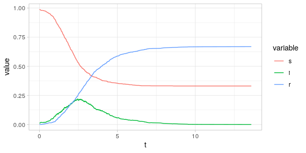
In the plot of the simulation, we see the stochastic effects in the \(s,i\) and \(r\) trajectories. Compare this, for example, with the trajectories produced by the deterministc model in my previous post: The SIR Model.

In a future post we will examine the effects that different degree distributions have on the dynamics of the networked SIR model, and use the SINDy framework to obtain a parsimonious (deterministic and continuous) differential equation model of the networked SIR dynamics given different degree distributions.

I hope you liked the post. Please leave any questions or comments in the commenting section below!

References

[Kiss et al., 2017] Kiss, I. Z., Miller, J. C. & Simon, P. L. Mathematics of epidemics on networks: From exact to approximate models. in Interdisciplinary Applied Mathematics vol. 46 1–413 (Springer, 2017).

[Gillespie, 1977] Gillespie, D. T. Exact stochastic simulation of coupled chemical reactions. J. Phys. Chem. 81, 2340–2361 (1977).