The Susceptible, Infected, Recovered (SIR) model

If you dabble in mathematical modeling, chances are that you (because of COVID-19) have been exposed to the SIR epidemiological model in the last year or two.

There is a wealth of material on the SIR model available online, so I will only cover the absolute basic points that are needed to aid understanding of the networked SIR model later on in this blog-post series. At least it well enable us to establish some notation.

The SIR model is a simple compartmental model of how an uncontrolled epidemic evolves in a population of size \(N\). I.e. it gives the change over time \( t \) (in the form of 3 coupled ODEs) of the fractions \(s(t)=S(t)/N,\,i(t)=I(t)/N\) and \(r(t)=R(t)/N\) of the population in the Susceptible (\(S(t)\)), Infected (\(I(t)\)) and Recovered (\(R(t)\)) compartments respectively at time \(t\), given that a certain fraction of the population is infected initially.

\[ \begin{split} \frac{d}{dt}\,s(t) = \dot s(t) &= -\beta \, s(t)\, i(t) \\ \frac{d}{dt}\,i(t) = \dot i(t) &= \beta \,s(t) \,i(t) - \gamma \,i(t) \qquad (1) \\ \frac{d}{dt}\,r(t) = \dot r(t) &= \gamma \, i(t) \\ \end{split} \]

where \( \beta > 0 \) is the infection rate, and \( \gamma > 0 \) is the recovery rate.
Note that \( s(t) + i(t) + r(t) = 1 \) is a conserved quantity, which also means that one of the equations is redundant (something we will make use of later when applying SINDy to stochastic simulations of the networked SIR model).

Even though the model is deterministic, a probabilistic interpretation can sometimes aid one's intuition.
The \(s,i\) and \(r\) fractions (dropping the dependence on \( t \)) can be viewed as the probabilities that an individual picked at random from the population belongs to the \(S,I\) or \(R\) compartments respectively. Hence, \(\frac{d}{dt}\,s = \dot s \) is the change in the \(s\) probability over an infinitesimal time interval \(dt\).

Taking this probabilistic view, we see that \(\dot s\) is negatively proportional to the probability of picking an \((S,I)\) pair of individuals at random (with replacement) from the population.

Because of conservation of probability (\(s+i+r=1\)), this quantity appears in the \( \dot i \) equation with positive sign, since \(S \rightarrow I \rightarrow R \) is the only trajectory an individual can take through the compartments.

In the standard SIR model an individual is permanently immune (or deceased) to the epidemic once recovered (in the \(R \) compartment). Therefore a recovered individual cannot end up in the \(S\) compartment again.

Hence individuals leaving the \(S\) compartment must enter the \(I\) compartment. Similarly, individuals leaving the \(I\) compartment at rate \(\gamma\) enter the \(R\) compartment at the same rate.

Basic analysis

It is easy to see, that in order for there to be an equilibrium, we need \(i(t)=0\).
Also, we see that in order for \( i(t) \) to be increasing (i.e. an outbreak) we must have

\[ \begin{split} \dot i > 0 & \implies \beta \,s \,i - \gamma \,i > 0 \\ & \implies \beta \,s \,i > \gamma \,i \\ & \implies s > \frac{\gamma}{\beta} \quad (0 < i \leq 1) \end{split} \]

Since \(s(t)\) is always less than 1 (when there is an epidemic), then the ratio \( \frac{\gamma}{\beta} \) must be less than 1 in order for it to be possible that \(i(t)\) be increasing at any time \(t\).
The ratio \( \frac{\gamma}{\beta} \) is the reciprocal of \(R_0\) — the basic reproductive ratio \( (R_0 = \frac{\beta}{\gamma}) \) [Kiss et al., 2017].

Ok, let's see some examples of the SIR model in action using R!

Code example

We can numerically integrate the ODE system in (1) using deSolve::ode. Below we are using \(\beta = 2\) and \(\gamma = 1\), with initial conditions \(s(0) = 0.99, i(0)=0.01,r(0)=0\).

Plot of the system in (1) produced by the supplied code snippet above.

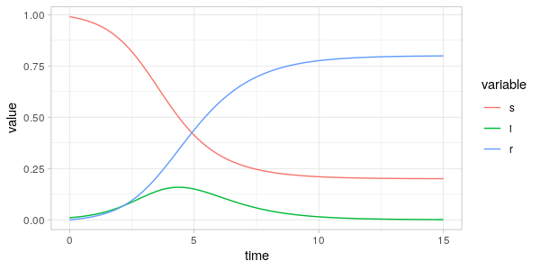
In the figure above we see the characteristic trajectories for the SIR model, when only a small fraction of the population is infected initially. We see that in this scenario approximately 80% of the population is infected at some time, with the maximum number of infected being around 16% for \(t\approx 4\).

This is all well and good, but let's return to our probabilistic interpretation of the SIR model above: There, \( \dot s \) is negatively proportional to the probability of picking an \( (S,I) \) pair, hence assuming that all individuals in the population may interact with each other. Otherwise there couldn't be any pathogen transmission resulting in infected individuals.

One might argue that this assumption is unrealistic, especially for large populations, and that this could be mitigated by letting the interactions be dependent upon a graph/network, that models which interactions are possible within the population.

This is exactly what is done in the networked SIR model. There, the individuals/agents are modelled as vertices in a graph, with interactions only being possible between vertices where there exists an edge (symmetric physio-social relation).
This is also where the modelling ceases to be deterministic and continuous. Instead transmission from an infected to a susceptible agent takes place as a Poisson process, i.e. a random or stochastic process, with rate \(\hat \beta\) — the per-edge infection rate, while recovery of agents is a Poisson process with rate \(\gamma\), independent of the graph [Kiss et al., 2017].

The networked SIR model which will be the subject of a future blog post, where we also cover how to do stochastic simulations of the same model using the Gillespie algorithm.

Stay tuned, and please leave your questions and comments in the commenting section below!

References

[Kiss et al., 2017] Kiss, I. Z., Miller, J. C. & Simon, P. L. Mathematics of epidemics on networks: From exact to approximate models. in Interdisciplinary Applied Mathematics vol. 46 1–413 (Springer, 2017).