Centrality Measures and The Networked SIR Model
Note: In this, and all posts in this series, the terms "graph" and "network" are used interchangeably. The same applies to the terms "node", "vertex" and "individual".
In this post I will be talking about how observations of network centralities, from simulations of the networked SIR model (previous post), may be used as predictors when applying the SINDy systems identification method (another previous post).
Centrality measures have been considered before in the literature in connection with the networked SIR model, for example in [Dekker, 2013],[Bucur et al., 2020] and [Yuan et al., 2013], but I have not seen papers where aggregates of centrality measures, for nodes in the different compartments, are tracked over the duration of a simulation, which is what we will be looking at here.
What is a network centrality measure?
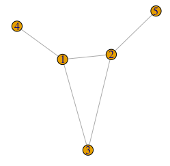
In the following let \(V\) be the vertex set of a finite graph \(G\), with cardinality \(|V|=N\).
Network centrality measures offer a way to quantify connectivity properties of a vertex \(v_j \in V\) according to some criteria. Depending on the application, the measure establishes the importance of the vertex from a connectivity standpoint.
Well known centrality measures include for example degree centrality, betweenness centrality, eigenvector centrality and closeness centrality amongst others.
For example, the degree centrality \( C_D(v_j) \)of a vertex \(v_j\) is the number of edges that are adjacent to the it, and so coincides with the vertex degree \( deg(v_j) \).
The betweenness centrality \(C_B(v_j)\) for \(v_j \in V\) is defined as the sum of the fractions of shortest paths (counting edges) in \(G\) going through \(v_j\) between all vertice pairs \(v_i,v_k \in V\), where \(i,k,j \in \{1,2,\ldots,N\}\) and \(i\neq j,\, i < k \neq j\), times a normalizing factor.
where \( \sigma_{ik}(j) \) denotes the number of shortest paths from \(v_i\) to \(v_k\) going through \(v_j\),
and \(\sigma_{ik}\) is the total number of shortest paths from \(v_i\) to \(v_k\) [Dekker, 2013].
The normalizing factor \(\frac{2}{(N-1)(N-2)}\) above corresponds to the one
used in the igraph package, when computing the betweenness centrality in R
(using igraph::betweenness with the normalized=TRUE option),
but one may come across other factors in the literature.
Betweenness centrality can for example be used to identify bottlenecks in traffic networks,
since traffic usually takes the shortest route from A to B.
Aggregates of centralities
In my master's thesis I wanted to find some way to use dynamic centrality observations from simulations as predictors when applying SINDy. My thinking was that an infected node's centrality measure, for example considering degree centrality, would clearly influence the time derivative target that we want to approximate when using SINDy. The solution I came up with, was to use the fraction of the centrality sum accounted for by the individuals in the \(S(t),\,I(t)\) and \(R(t)\) vertex sets at time \(t\). If I may elaborate...
Let \( C_*(v_i) \) be any per-node centrality measure for a graph \(G\) with \(v_i \in V \), then \( C_*(G) = \sum_{j=1}^N C_*(v_j) \) is a graph invariant. The quatity
is an \(s(t)\)-like trajectory, but in terms of a fraction of a graph invariant, instead of fraction of a population. The case being similar for the \(i_C(t)\) and \(r_C(t)\) fractions. Depending on the measure \(C_*\) being used, the different centrality-sum fractions (CSFs) above provide dynamical information about how the pathogen in the networked SIR model is spreading through the population from a topological standpoint. It is somewhat unclear exactly what information is being conveyed, but the assumption is that the information is useful in a machine learning context, i.e using SINDy.
Another thing to consider, is that a model of the networked SIR dynamics using CSFs as predictors will have more than 3 equations — one additional for every CSF used as a predictor,
unless one assumes that the CSFs are known functions of time,
which would render the model less useful in an applied sense.
The good news is, that the sum of CSFs is a conserved quantity, i.e. \(s_C + i_C + r_C = 1\),
which enables us to use som "tricks" when finding a model with SINDy.
More on this in the final post in this series.
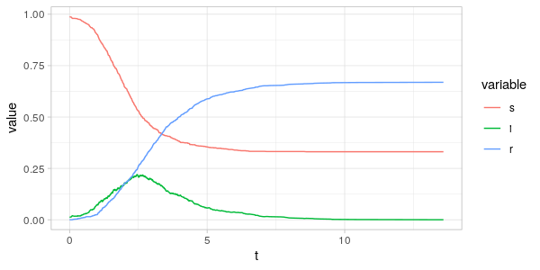
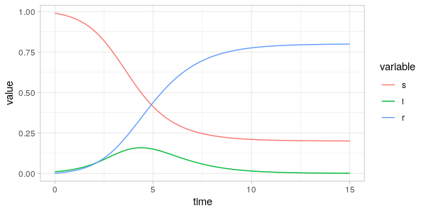
Simulation example
Let's see what these CSF trajectories look like when using degree centrality and betweenness centrality.
I've made a small modification to the networked-sir.R code from the previous post.
The networked_sir() function now takes an additional vector C as an argument which
gives some per-vertex centrality measure. The CSFs are then computed using the csf() function,
and returned in observation data frame. In the simulation below, we use degree centrality and betweenness centrality respectively.
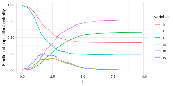
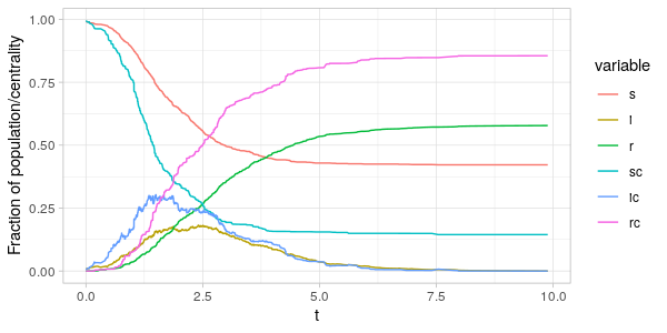
As can be seen from the plots above the fraction of the centrality-sum
accounted for by the nodes in the \(S(t),I(t)\) and \(R(t)\) vertex sets
are far from the same as the fraction of population in the same sets.
Comparing \(i(t)\) and \(i_C(t)\) in the two plots, we see that around the peak of the epidemic
it is the nodes with high degree and betweenness that are infected.
Since an infected node with many edges (high degree) is likely to increase the infection rate of many susceptible neighbours,
and thereby likely the estimated derivative of \(i(t)\) and \(s(t)\), it seems natural to use the degree-CSFs as
predictors in regression where the target is the estimated derivative (i.e. the SINDy stage).
The case is not so clear for betweenness-CSFs, since a vertex can have high betweenness but low degree.
Even so, CSFs using degree and betweenness centrality are strongly correlated ( \( \approx 0.97 \) for the two \(i_C(t) \) time-series above).
Conclusion
It appears that using CSFs provides us with additional information about how a pathogen spreads through
a population in the networked SIR model.
In the next post I will be using CSFs as predictors in sparse regression when using SINDy,
and leave it up to the LASSO algorithm to decide whether the CSF predictors should be included in the resulting model.
References
[Dekker, 2013] Dekker, A. H. Network centrality and super-spreaders in infectious disease epidemiology. Proc. - 20th Int. Congr. Model. Simulation, MODSIM 2013 331–337 (2013) doi:10.36334/modsim.2013.a5.dekker.
[Bucur et al., 2020] Bucur, D. & Holme, P. Beyond ranking nodes: Predicting epidemic outbreak sizes by network centralities. PLoS Comput. Biol. 16, 1–20 (2020).
[Yuan et al., 2013] Yuan, C., Chai, Y., Li, P. & Yang, Y. Impact of the network structure on transmission dynamics in complex networks. IFAC Proc. Vol. 13, 218–223 (2013).